

Flexible capacitor, part 5: Comparison with analytical solution
[latexpage]
In the previous tutorial in this series, we modified the program to automatically ensure that the boundary of the capacitor was circular whenever it was refined. Our script now solves the original problem posed in the first tutorial, namely to solve for the electric potential inside circular capacitor with four electrodes. 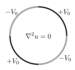
We’re now therefore ready to assess our solution. Fortunately, this problem is sufficiently simple that an analytical solution is available in the form of a series,
$$u(r,\theta) = \sum_{i=1}^{\infty} \frac{4 w r^{4 n+2} \sin (\theta (4 n+2))}{\pi (2 n+1) (4 n+w+2)}$$
where $w=\frac{W}{\epsilon0}$ is the ratio of prefactors in front of the boundary energy and electrostatic energies. As $w$ becomes large, the boundary condition is enforced more strongly, and as $w\to\infty$ the boundary condition approaches a Dirichlet boundary condition. Note that the solution here is expressed in 2D polar coordinates.
The code for this tutorial is given below, which includes all the necessary new functions. Cut and paste into a text file and run with Morpho; you’ll still need the ‘disk.mesh’ file from previous tutorials.
[code lang=”js” gutter=”false” collapse=”true” title=”Compare with analytical solution”]
/* —————————————————————
* Capacitor with adaptive refinement
* ————————————————————— */
/* —————————————————————
* Control parameters
* ————————————————————— */
Nsteps = 50 // Number of steps to take on the initial minimization
Nsteps2= 200 // Number of minimization steps to take for each level of refinement
Nlevels=4 // Number of levels of refinement
V0=1 // The potential at both electrodes
W=1 // The prefactor in front of the anchoring term
/* —————————————————————
* Load manifold and apply all the energies
* ————————————————————— */
// Set up the colormap for plotting
@mymap = {
redcomponent(x) = 0.29+0.82*x-0.17*x^2;
greencomponent(x) = 0.04+1.66*x-0.79*x^2;
bluecomponent(x) = 0.54+1.18*x-0.9*x^2;
}
cm=new(mymap);
// Obtain the initial mesh
m=manifoldload("disk.mesh")
// Select the boundary
boundary=m[1].selectboundary()
// Upper and lower boundary for anchoring
electrode1=m.select(x^2+y^2>0.99 && ((x>-0.1 && y>-0.05) || (x<0.1 && y<0.05)), coordinates={x,y,z}, grade={0,1});
electrode2=m.select(x^2+y^2>0.99 && ((x<0.1 && y>-0.05) || (x>-0.1 && y<0.05)), coordinates={x,y,z}, grade={0,1});
// Create a field on the manifold
V=m.newfield(x*y, coordinates={x,y,z});
lc=new(electrostatic);
lc.setfield(V);
m.addenergy(lc)
// Impose a harmonic constraint on the boundaries
lh=new(fieldharmonic);
lh.setfield(V);
lh.setvalue(1);
lh.setprefactor(W);
m.addenergy(lh, electrode1)
lh2=new(fieldharmonic);
lh2.setfield(V);
lh2.setvalue(-1);
lh2.setprefactor(W);
m.addenergy(lh2, electrode2)
/* —————————————————————
* Set up functions that will automate various tasks for us
* ————————————————————— */
//Minimization
minimize(a, n) = {
table(
a.linesearchfield();
en=a.totalenergy();
// print(en);
en
,{i, n}
)
}
// Show histogram
showhist(a, func) = {
histogram(func.integrand(a[1]).tolist())
}
// Adaptive refinement
adaptiverefine(a, mult, func) = {
f = func.integrand(a[1]);
threshold=mult*f.total()/length(f.tolist());
g = f.map(function(x, x>threshold));
p = a.select(g).changegrade({0,1});
a.refine(p);
a[1].equiangulate();
};
/* —————————————————————
* Reproject boundaries onto the unit circle using a listener
* ————————————————————— */
// Normalizes a vector given as a list by dividing throughout by the norm
normalize(list) = {
norm=sqrt(sum(list[i]^2, {i,length(list)}));
table(list[i]/norm, {i,length(list)})
}
// circularize
@circularizer = {
update(manifold, result) = {
bnd = manifold.selectboundary(); // Creates a selection with the boundary elements and vertices
ids = bnd.idlistforgrade(manifold, 0); // Obtains a list of vertex ids
do(
posn=manifold.vertexposition(ids[i]); // Gets the position of the vertex i
manifold.setvertexposition(ids[i], normalize(posn)) // normalizes the position and sets it
,{i,length(ids)}
);
m.changed(); // Tell the body that the manifold has changed to ensure the display is updated
}
}
// Instantiate a circularizer object
circ=new(circularizer);
// Have this object listen to the refine selector of the manifold
m[1].addlistener(circ, refine, update);
/* —————————————————————
* Analytical solution
* ————————————————————— */
// Term in the series solution for the potential
term(x, y, W, n) = {
nn=4*n+2;
r=sqrt(x^2+y^2);
theta=arctan(x,y);
bc=4/(2*n+1);
bc*r^nn*sin(nn*theta)*W/pi/(nn+W)
}
// Term in the series solution for the electrostatic energy
esterm(W, n) = {
nn=4*n+2;
bc=4/(2*n+1);
cn=bc*W/pi/(nn+W);
cn^2*nn*pi
}
// Term in the series solution for the boundary energy
bterm(W, n) = {
nn=4*n+2;
bc=4/(2*n+1);
cn=bc*W/pi/(nn+W);
cn^2*pi – 4*cn*(1+(-1)^nn – 2*cos(nn*pi/2))/nn
}
// Calculate the rms value of a list
rms(list) = sqrt(sum(list[i]^2,{i,length(list)}))/length(list)
// Evaluate the analytical potential at a point
Vana(x,y) = sum(term(x,y,W,n),{n,0,400})
// Evaluate the analytical electrostatic energy
Esana = sum(esterm(W,n),{n,0,400})
// Evaluate the analytical boundary energy
Bana = 2*pi + sum(bterm(W,n),{n,0,400})
// Display a report of the error
assesserror() = {
Ecomp=lc.total(m[1]);
Bcomp=lh.total(m[1],electrode1)+lh2.total(m[1],electrode2);
print("Electrostatic energy calculated:", Ecomp, " analytical:", Esana," diff:", Ecomp-Esana," rel. error:", (Ecomp-Esana)/Esana);
print("Boundary energy calculated:", Bcomp, " analytical:", Bana," diff:", Bcomp-Bana," rel. error:", (Bcomp-Bana)/Bana);
Vcomp=m.newfield(Vana(x,y), coordinates={x,y,z});
err=(Vcomp-V).tolist();
print("RMS error = ",rms(err), " with ",length(err), " degrees of freedom.");
histogram(err);
print();
}
/* —————————————————————
* Main work
* ————————————————————— */
show(m)
tt1=minimize(m, Nsteps);
assesserror();
tt2=table(
adaptiverefine(m, 1.0, lc);
ttx=minimize(m, Nsteps2);
assesserror();
ttx
, {i,Nlevels}
);
show(m.draw(V, colormap=cm))
[/code]
When you run the program, you’ll see Morpho solve and refine as in the previous tutorial, but at every level of refinement Morpho will also print a report comparing various features of the solution with the analytical results above. For example, after the first iteration you’ll see something like this:
[code lang=”js” gutter=”false”]
Electrostatic energy calculated:1.11019 analytical:1.23341 diff:-0.123222 rel. error:-0.0999033
Boundary energy calculated:3.55258 analytical:3.23642 diff:0.316155 rel. error:0.0976865
RMS error = 0.00245363 with 29 degrees of freedom.
-0.0240485 – -0.0144291 : 4
-0.0144291 – -0.0048097 : 6
-0.0048097 – 0.0048097 : 9
0.0048097 – 0.0144291 : 6
0.0144291 – 0.0240485 : 4
[/code]
There’s a lot of information here, so let’s go through it step by step. First, let’s look at the energy. Inserting the above solution into the expressions for the energy, i.e. $\int_C (\nabla u)^2 dA$ and $\int_{\partial C} (u-u_0)^2 dl$, it’s possible to obtain the following series that evaluates to the electrostatic energy and boundary energy respectively:
$$E_{electrostatic} = \sum_{i=1}^{\infty} \frac{32 W^2}{(2 \pi n+\pi ) (4 n+W+2)^2}$$
$$E_{boundary} = 2\pi – \sum_{i=1}^{\infty} \frac{16 W (8 n+W+4)}{\pi (2 n+1)^2 (4 n+W+2)^2}$$
For the parameter $W=1$, we get the analytical values $E_{electrostatic} = 1.23341$ and $E_{boundary} = 3.23642$. At each level of refinement, our program reports the discrepancy between the calculated value of the energy from the solution and these analytical values, as well as the relative error i.e. $|E_{soln}-E_{analytical}|/E_{analytical}$.
We can plot the relative error as a function of the number of degrees of freedom for both the boundary and electrostatic terms:
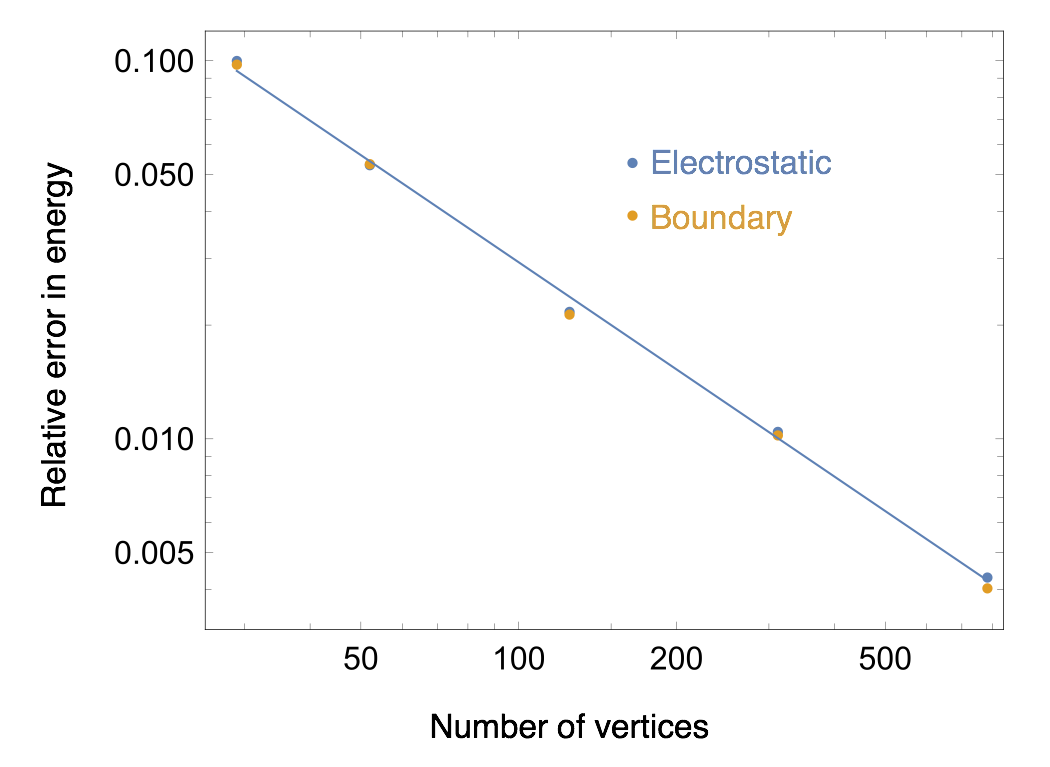
These are plotted on log-log scales showing a linear trend indicative of a power law relationship between the relative error and the number of vertices. Fitting the data to a linear model gives the value of the power as $~1$, which is the relationship expected for linear elements. So far so good!
We’ll now look at the local error in the solution. There are more sophisticated ways of measuring this, but for now let’s just look at the point wise difference between the analytical and calculated value and compute the root mean squared (RMS) value. The program also outputs a histogram of the distribution so you can get a sense of how the distribution changes, and in particular the absolute bounds on the error.
Below, we show the maximum and RMS errors as a function of the number of mesh points. It’s interesting to note that while the RMS error decreases $\propto N^{-1.33}$, the maximum error only decreases $\propto\sqrt N$. This relatively poor performance motivates other discretizations, as we’ll discuss in later tutorials.
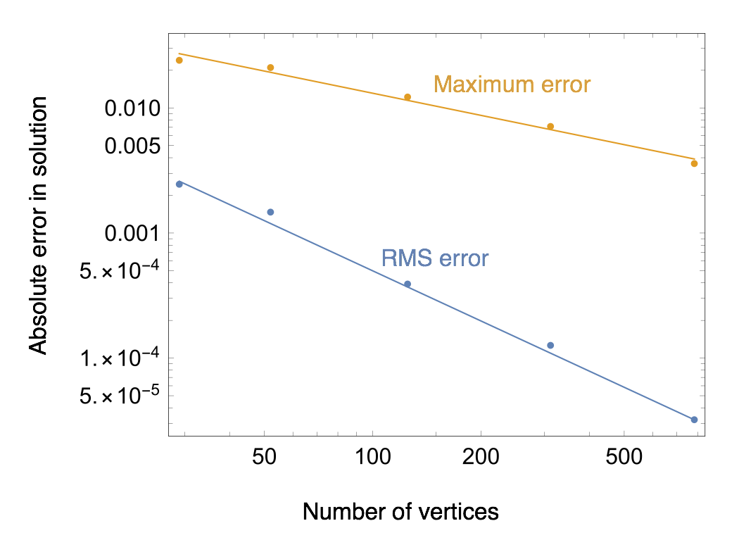
The good news is that Morpho is clearly converging on the correct solution as $N$ increases, and this analytically solvable test case is therefore a valuable check to verify everything is working properly. In the next tutorial, we’ll make the capacitor flexible, and hence solve the original problem.
Exercise 1 How does the error in the energy and solution change if $W$ is altered? Try adjusting this parameter and rerunning the program.
Exercise 2 Above we used the adaptive refinement strategy from tutorial 3 in this series. What happens if you replace this refinement strategy with regular refinement? Do you get the same scaling with $N$?