Flexible capacitor, part 2: Visualizing and solving for the electric potential

[latexpage]
In the first tutorial in this sequence, we loaded an initial mesh for the capacitor problem and learned how to select the boundary and electrodes. In this tutorial, we will create the electric potential field, define the energy functional that we want to minimize and solve for the potential on our mesh. The code for this tutorial will get quite long, so to save typing it in repeatedly, create a new plain text file to hold the script, copy and paste the below and save it as “capacitor.morpho”.

[code lang=”js” gutter=”false”]
// Obtain the initial mesh
m=manifoldload("disk.mesh")

// Select the boundary
boundary=m[1].selectboundary()

// Upper and lower boundary for anchoring
electrode1=m.select(x^2+y^2>0.99 && ((x>-0.1 && y>-0.05) || (x<0.1 && y<0.05)), coordinates={x,y,z}, grade={0,1});
electrode2=m.select(x^2+y^2>0.99 && ((x<0.1 && y>-0.05) || (x>-0.1 && y<0.05)), coordinates={x,y,z}, grade={0,1});
[/code]

Make sure you start Morpho from the directory in which this script is saved, and then you can run the script from within Morpho by typing

[code lang=”js” gutter=”false”]
run("capacitor.morpho")
[/code]

We’re now ready to amend the script. Our first task is to create the electric potential. The method to do this is newfield() and the way to use this is very similar to the select() method used in the preceding tutorial:

[code lang=”js” gutter=”false”]
V=m.newfield(y, coordinates={x,y,z});
[/code]

This line of code creates a new field on the body m, with an initial value defined by the function $V(x,y)=x y$. The option coordinates just tells Morpho which variables correspond to which coordinates, and hence allows us the freedom to rename the coordinate names if we so choose. If you execute this, you’ll see that the variable V now contains a reference to a field object, which hopefully should be an encouraging sign!

To visualize this initial potential, we can just supply the field as an argument to the draw() method

[code lang=”js” gutter=”false”]
show(m.draw(V))
[/code]

which should produce a plot that looks like this:

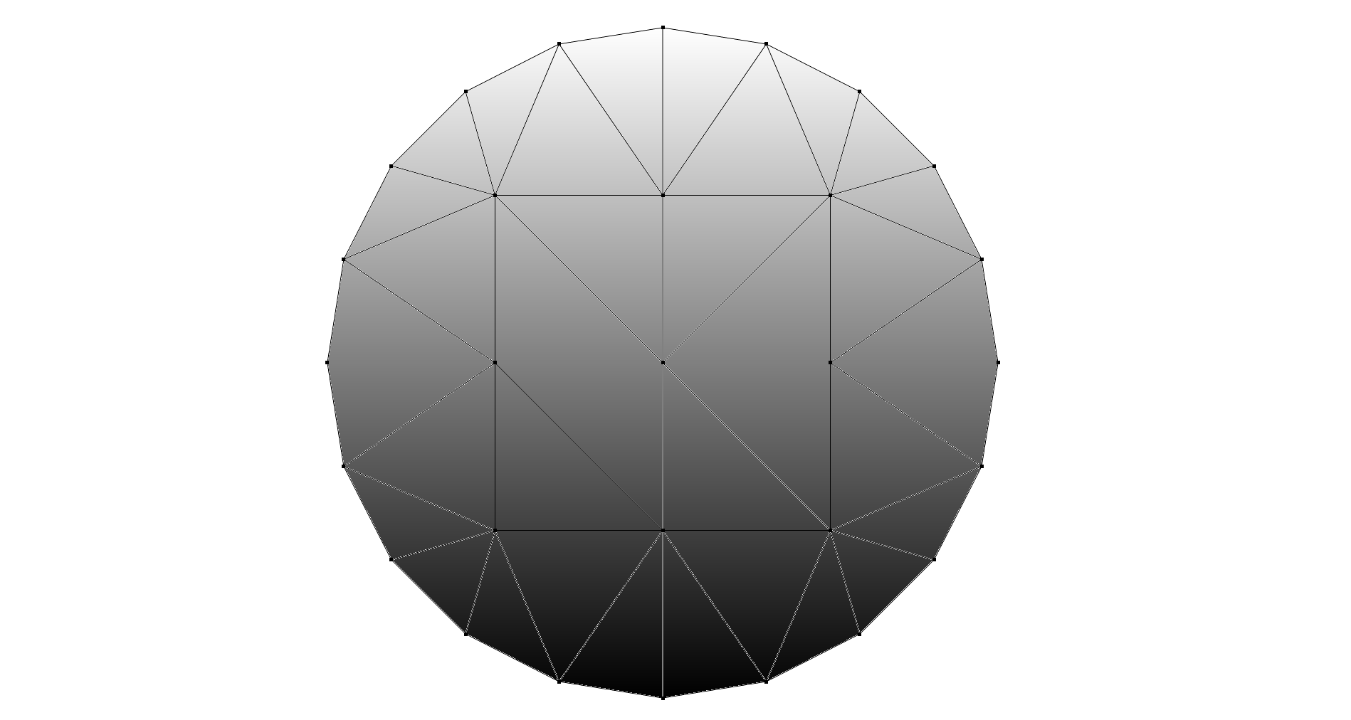
Here the values of the electric potential are visualized as a grayscale shading of the mesh. We can use different color schemes by defining an object that responds to the colormap protocol. For example, if you insert the following code before the call to draw,

[code lang=”js” gutter=”false”]
// Set up the colormap for plotting
@mymap = {
redcomponent(x) = 0.29+0.82*x-0.17*x^2;
greencomponent(x) = 0.04+1.66*x-0.79*x^2;
bluecomponent(x) = 0.54+1.18*x-0.9*x^2;
}

cm=new(mymap);
[/code]

This defines a class called mymap that responds to three methods redcomponent, greencomponent, bluecomponent, each of which accept a scalar argument—here the value of the electric potential—and map it to a color value. The call to new instantiates a mymap object ready for use.

We can now supply the colormap object as an option to draw(),

[code lang=”js” gutter=”false”]
show(m.draw(V, colormap=cm))
[/code]

which should produce a more colorful plot:

We’re now ready to define the electrostatic energy, which is given by the integral $\int_C (\nabla u)^2 dA$ where $u$ is the electric potential and the domain of integration is over the entire capacitor $C$. The necessary code in Morpho is

[code lang=”js” gutter=”false”]
lc=new(electrostatic);
lc.setfield(V);
m.addenergy(lc)
[/code]

This first creates a new electrostatic object, calls setfield() to tell it that the field V is the electric potential, and then adds it to the list of energies to be minimized.

One can see what the current value of the energy is by typing

[code lang=”js” gutter=”false”]
m.totalenergy()
[/code]

which should produce $1.63872$ if everything has been set up properly as above.

It’s now necessary to specify the boundary conditions for the electric potential. It’s very common in electrostatic problems to impose a fixed value of V on the boundary, leading to what is known as a Dirichlet boundary condition. This is possible in Morpho, but generally causes pathologies for shape change problems. Notably, sudden changes in the values of the potential on the boundary (such as occur between the electrodes) lead to discontinuous shapes. Here we demonstrate a gentler boundary condition, where instead we allow the value of the potential on the boundary to vary, but penalize the difference between its value and some preferred value $u_0$. The energy to be minimized is therefore $\int_{\partial C} (u-u_0)^2 dl$.

To do this in Morpho, we write

[code lang=”js” gutter=”false”]
// Impose a harmonic constraint on the boundaries
lh=new(fieldharmonic);
lh.setfield(V);
lh.setvalue(1);
m.addenergy(lh, electrode1)

lh2=new(fieldharmonic);
lh2.setfield(V);
lh2.setvalue(-1);
m.addenergy(lh2, electrode2)
[/code]

which, for each electrode in turn, creates a fieldharmonic object, tells it that V is the field to use, sets $\pm1$ as the preferred value and adds it to the list of energies. Note that in addenergy() the selections are included to restrict the energy only to the separate electrodes.

Having specified all these energies, we’re now ready to perform the minimization. Let’s begin by checking what the total energy is by typing,

[code lang=”js” gutter=”false”]
m.totalenergy()
[/code]

which should give a value of $4.77683$. We can take one minimization step in the electric potential values by typing

[code lang=”js” gutter=”false”]
m.linesearchfield()
[/code]

which is closely related to the linesearch() method used in earlier tutorials. The linesearch() method moves the mesh to reduce the energy, linesearchfield() reduces the energy my changing the field.

Exercise 1  Check on the new value of the total energy. Has it decreased? By how much?

We can further minimize the energy by calling linesearchfield() repeatedly until the energy doesn’t change any further. It’s easiest to do this using a loop. For this small mesh, 30 iterations is sufficient.

[code lang=”js” gutter=”false”]
do(
m.linesearchfield();
print(m.totalenergy());
,{i,30})
[/code]

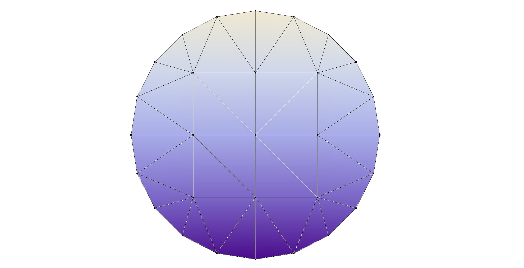
Notice the energy converges on a final value $4.66276$. We can now visualize the minimized electrostatic potential by typing

[code lang=”js” gutter=”false”]
show(m.draw(V, colormap=cm))
[/code]

which should produce:

This solution looks very plausible as it has the correct symmetry imposed by the electrodes, but it’s on a very coarse mesh. In the next tutorial, we’ll refine the mesh and improve the solution.

Exercise 1  Plot the energy as a function of iteration to determine how the solution converges. Hint: Take a look at this previous tutorial. You may like to try plotting the log of $E_i – E_f$ as a function of iteration, where $E_i$ is the value after the $i$th iteration and $E_f$ is the value after the final iteration. This plot should look like a straight line, showing that the solution is converging exponentially.

Exercise 2  You can enforce the boundary conditions more strongly by calling setprefactor for each boundary energy right after the lines lh.setvalue(1); and lh2.setvalue(1); for electrodes 1 and 2 respectively. The setprefactor method takes a single argument that’s the coefficient in front of the integral. The default value is 1. What happens to the solution if you use other values such as $10$ and $0.1$?

[code lang=”js” gutter=”false” collapse=”true” title=”Solution to Exercise 1″]
t=table(
m.linesearchfield();
m.totalenergy()
,{i,30});

v=table({i,log(t[i]-t[30])},{i,length(t)-1})

plotlist(v).export("energyconvergence.eps")
[/code]