

Flexible capacitor, part 3: Refinement
[latexpage]
In the previous tutorial in this sequence, we set up the electric potential for our capacitor, defined the electrostatic energy in our calculation and applied a harmonic boundary condition. We then minimized the energy, solving the problem on our initial mesh. While this worked fine, the mesh we used only had a few vertices (29 to be exact!) and so the resulting solution cannot be very accurate. During this tutorial, you’ll learn how to add additional mesh points to produce a better solution.
Before we begin, it’s worth restating the script we developed in previous tutorials. I’ve tidied it up a bit, and used comments to divide it into functional blocks, which is highly recommended as scripts get longer. Further, some of the key parameters for the script are defined at the start to make it easier to change. I also created a function called minimize that runs linesearchfield a specified number of times. Copy the below into a text editor and save it as a new script “capacitorpart3.morpho”.
[code lang=”js” gutter=”false” collapse=”true” title=”Flexible Capacitor script, version 3″]
/* —————————————————————
* Flexible capacitor
* ————————————————————— */
/* —————————————————————
* Control parameters
* ————————————————————— */
Nsteps = 30 // Number of steps to take on the initial minimization
V0=1 // The potential at both electrodes
W=1 // The prefactor in front of the anchoring term
/* —————————————————————
* Load manifold and apply all the energies
* ————————————————————— */
// Set up the colormap for plotting
@mymap = {
redcomponent(x) = 0.29+0.82*x-0.17*x^2;
greencomponent(x) = 0.04+1.66*x-0.79*x^2;
bluecomponent(x) = 0.54+1.18*x-0.9*x^2;
}
cm=new(mymap);
// Obtain the initial mesh
m=manifoldload("disk.mesh")
// Select the boundary
boundary=m[1].selectboundary()
// Upper and lower boundary for anchoring
electrode1=m.select(x^2+y^2>0.99 && ((x>-0.1 && y>-0.05) || (x<0.1 && y<0.05)), coordinates={x,y,z}, grade={0,1});
electrode2=m.select(x^2+y^2>0.99 && ((x<0.1 && y>-0.05) || (x>-0.1 && y<0.05)), coordinates={x,y,z}, grade={0,1});
// Create a field on the manifold
V=m.newfield(x*y, coordinates={x,y,z});
lc=new(electrostatic);
lc.setfield(V);
m.addenergy(lc)
// Impose a harmonic constraint on the boundaries
lh=new(fieldharmonic);
lh.setfield(V);
lh.setvalue(1);
lh.setprefactor(W);
m.addenergy(lh, electrode1)
lh2=new(fieldharmonic);
lh2.setfield(V);
lh2.setvalue(-1);
lh2.setprefactor(W);
m.addenergy(lh2, electrode2)
/* —————————————————————
* Set up functions that will automate various tasks for us
* ————————————————————— */
//Minimization
minimize(a, n) = {
table(
a.linesearchfield();
en=a.totalenergy();
print(en);
en
,{i, n}
)
}
/* —————————————————————
* Main section
* ————————————————————— */
[/code]
Now launch Morpho from the directory you saved it in and type
[code lang=”js” gutter=”false”]
run("capacitorpart3.morpho")
tt1=minimize(m, Nsteps);
show(m.draw(V, colormap=cm))
[/code]
and the resulting solution from the previous tutorial should appear:

We can refine the model simply by typing
[code lang=”js” gutter=”false”]
m.refine()
[/code]
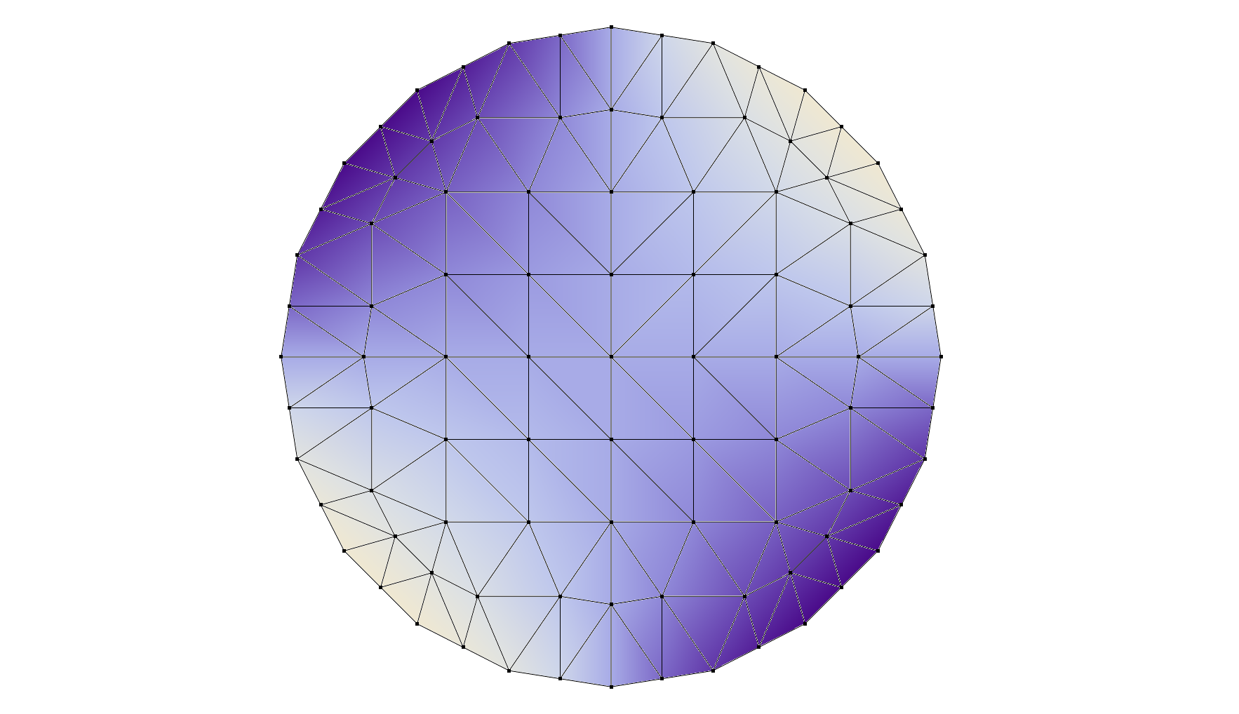
which divides every single triangle into four new triangles by bisecting each of the sides. This leads to a representation of the solution with 93 vertices. Because we packaged up the minimization loop into a function, re-minimizing the energy is as easy as
[code lang=”js” gutter=”false”]
tt2=minimize(m, 100);
show(m.draw(V, colormap=cm))
[/code]
where you’re free to change the number 100 to anything you want. What we’re looking for is an indication that the solution has converged, i.e. the energy doesn’t change any further. After running this, you’ll see the refined solution:
Exercise 1 Call refine again and re-minimize. Notice that Morpho slows down for each iteration as many more quantities have to be computed. Visualize the solution.
Exercise 2 What happens if you re-run the script, but now call m.refine() twice before doing any minimization? You should find that the solution still converges, but takes much longer to run because, after all, it has so many more vertices. This is why we use the strategy of minimize$\to$refine$\to$minimize$\to$refine, known as successive refinement, because we save a lot of unnecessary calculation.
The above strategy of refining the entire mesh is, however, still quite wasteful as clearly the electric potential is nearly constant in the middle of the capacitor. Morpho provides the ability to refine only selected portions of a mesh, and a good criterion to use is the energy contained in each element. We would obviously like to refine those elements that contain the most energy.
Let’s begin again with our coarse mesh. Type:
[code lang=”js” gutter=”false”]
run("capacitorpart3.morpho")
tt1=minimize(m, Nsteps);
show(m.draw(V, colormap=cm))
[/code]
and you should see the coarse solution once again.
We can obtain the energy contribution from each area element in the mesh by using a method from the electrostatic object. Type
[code lang=”js” gutter=”false”]
energydensity=lc.integrand(m[1])
[/code]
which creates a new field, energydensity, that contains an energy value for each area element in the mesh. It’s quite helpful to get a sense of the distribution of values in the field; to do so type
[code lang=”js” gutter=”false”]
histogram(energydensity.tolist())
[/code]
which outputs all the values in the field as a (randomly ordered) list, and then calls histogram to output a simple text-based histogram of the values:
[code lang=”js” gutter=”false”]
1.98132e-25 – 0.0119543 : 1
0.0119543 – 0.0239086 : 18
0.0239086 – 0.0358628 : 8
0.0358628 – 0.0478171 : 1
0.0478171 – 0.0597714 : 8
[/code]
Looking at the above, it seems like it might be a good idea to refine elements that have an energy greater than about 0.024. To do this, type
[code lang=”js” gutter=”false”]
test=energydensity.map(function(x, x>0.024))
[/code]
This creates a new field, test, which for every entry in energydensity contains an equivalent entry containing true or false depending on wether that entry was larger or smaller than 0.024. The intrinsic function is how Morpho constructs an anonymous function. This function is called for every entry in energydensity with the entry as the argument.
We can now use this field to make a selection,
[code lang=”js” gutter=”false”]
sel=m.select(test)
[/code]
It’s worth visualizing this selection,
[code lang=”js” gutter=”false”]
show(m.draw(sel))
[/code]
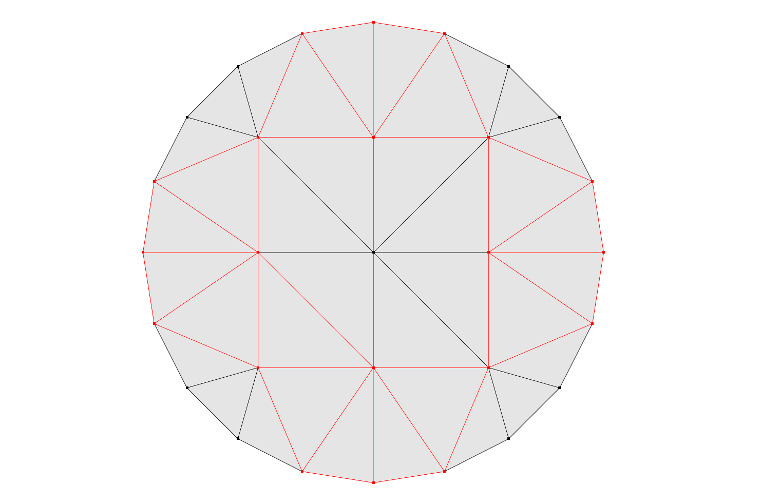
which should produce:

As we might expect from the earlier visualization of the field, the triangles closest to the electrode edges are the ones with highest energy, and hence should be refined. We can give m.refine() a selection object to do this, but a minor detail is that the selection needs to include vertices and lines–Morpho refers to these as grade 0 and grade 1 elements respectively–rather than points. We can easily achieve this with
[code lang=”js” gutter=”false”]
sel=m.select(test).changegrade({0,1})
[/code]
If you visualize this, you will see that the boundary edges and vertices from the earlier selection have been selected
We’re now ready to do the refinement. It’s as easy as
[code lang=”js” gutter=”false”]
m.refine(sel)
[/code]
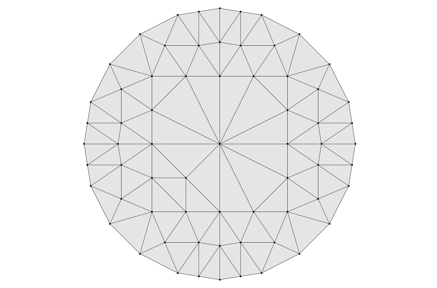
The mesh now looks like this:

One issue that comes up is that refinement occasionally produces some rather elongated triangles, which lead to poor numerical behavior. It’s a good idea to follow a selective refinement with a call to equiangulate
[code lang=”js” gutter=”false”]
m[1].equiangulate()
[/code]
which flips edges around to remove the long triangles.
We can now re-minimize the field,
[code lang=”js” gutter=”false”]
minimize(m, 100)
show(m.draw(V, colormap=cm))
[/code]
and see the result
 .
.
We’ll now wrap up the adaptive refinement into a convenient function just as we did for minimize. The complete script is included in the Morpho examples repository as “capacitorpart3.morpho”.
We add a couple of new functions to the section labelled ‘Set up functions that will automate various tasks for us’
[code lang=”js” gutter=”false”]
// Show histogram
showhist(a, func) = {
histogram(func.integrand(a[1]).tolist())
}
// Adaptive refinement
adaptiverefine(a, mult, func) = {
f = func.integrand(a[1]);
threshold=mult*f.total()/length(f.tolist());
g = f.map(function(x, x>threshold));
p = a.select(g).changegrade({0,1});
a.refine(p);
a[1].equiangulate();
[/code]
Here, the adaptiverefine function is a bit more sophisticated from our ‘eyeballing’ of the histogram: it calculates the mean value of the field and selects all elements that are mult times greater than the mean for refinement.
We also change the “Main section” code to call adaptiverefine and reminimize.
[code lang=”js” gutter=”false”]
show(m)
tt1=minimize(m, Nsteps);
showhist(m, lc)
tt2=table(
adaptiverefine(m, 1.0, lc);
ttx=minimize(m, Nsteps);
showhist(m, lc);
ttx
, {i,3}
);
show(m.draw(V, colormap=cm))
[/code]
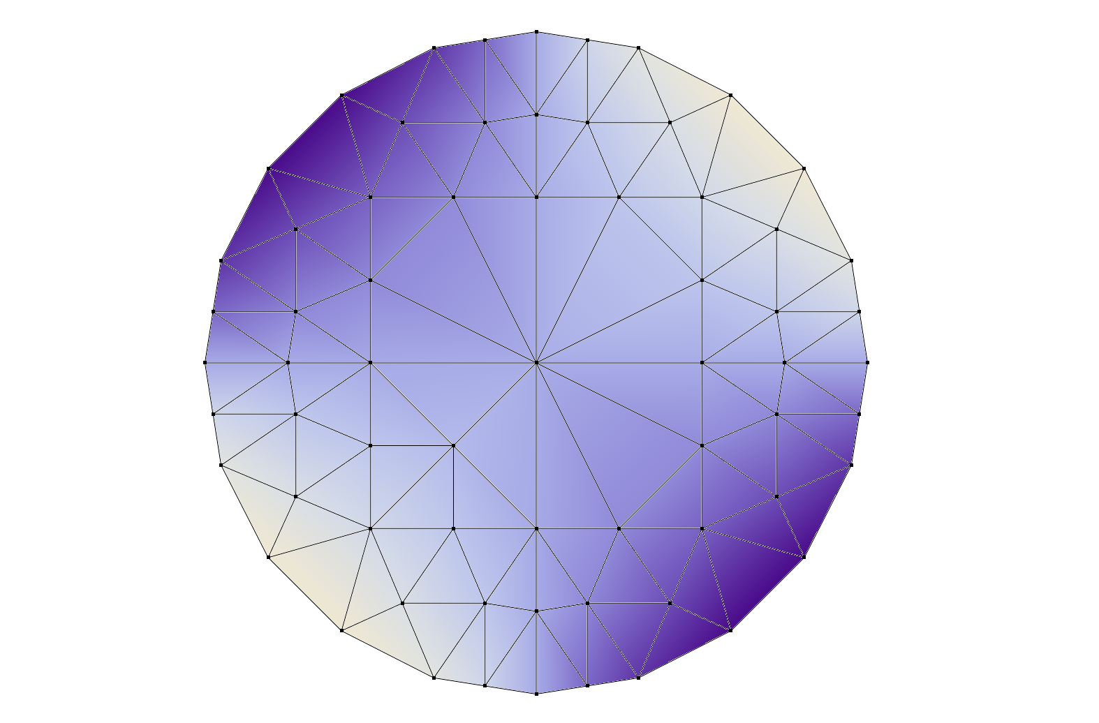
If you run the complete code, you’ll get the beautifully refined solution below. One problem that remains is that when the mesh is refined, the new boundary vertices are not on the unit circle. We’ll fix this in the next tutorial.

Exercise 3 Try adjusting the value of mult (initially) 1.0 in the call to adaptiverefine above. Try values from 0 to 2. How does each change the solution?