
Minimizing the length of a loop, part 4: Comparing the two approaches
In the previous post in this sequence of tutorials, we minimized the length of a loop at constant area and made sure that our solution was “good” in the sense of promoting equal length elements. There’s a very interesting side effect of the regularization that’s important to note, and we’ll explore it in this tutorial. What we’re going to do is to run the two minimizations side by side and compare how the total energy changes for each one.
To do this, we’ll use the following script:
[code lang=”js” gutter=”false”]
/* Minimize the length of a loop at constant area */
np=20 // Number of points
A=0.5 // Amplitude of initial distortion
Nsteps=100 // Number of steps to take
// Create the manifold
m=manifoldline({(1+A*cos(4*t))*cos(t), (1+A*cos(4*t))*sin(t),0}, {t,0,2*pi-pi/np/2, pi/np}, closed=true)
m2=manifoldline({(1+A*cos(4*t))*cos(t), (1+A*cos(4*t))*sin(t),0}, {t,0,2*pi-pi/np/2, pi/np}, closed=true)
// Add line tension
lt=new(linetension)
m.addenergy(lt)
m2.addenergy(lt)
// Keep the area enclosed constant
la=new(enclosedarea)
m.addconstraint(la)
m2.addconstraint(la)
//Promote equal sized segments
le=new(equilength);
m2.addregularization(le);
// Perform the minimization
t=table(
m.linesearch();
m.totalenergy()
, {i,Nsteps});
t2=table(
m2.linesearch();
m2.linesearch(le);
log(m2.totalenergy()
, {i,Nsteps});
p=plotlist({t,t2})
p.export("energy.eps")
[/code]
There are a number of important things to note here. First, while we create two identical manifolds, there’s no need to create a duplicate set of functionals. We can use the same functional objects for both. Second, rather than performing the minimization using do, we’re instead using table which creates a list of whatever it’s argument evaluates to. Notice that the last command in the minimization loop is a call to totalenergy() and the semicolon is omitted. This means that we’ll make a table of the total energy of the manifold at each iteration.
Exercise 1Run the script and examine its output by looking at what’s stored in t and t2. You should see a list of energy values.
The remaining two lines create a plot of the two lists of energy values and export it as an encapsulated postscript (EPS) file. If you look in the directory that you ran the script from, you should see a file “energy.eps” which if you open it looks like this:
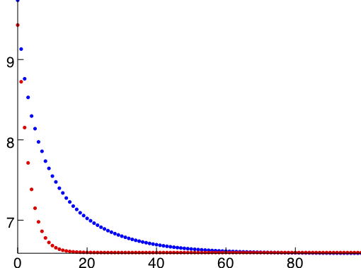
The blue curve is the first minimization, and the red curve is the second. Clearly, the regularized minimization converges much more rapidly. This is often found to be the case with Morpho, and is a good reason to use regularization. While regularization requires more computational effort per iteration, it typically repays this with faster convergence.
Exercise 2 Investigate this phenomenon further. Try plotting the result on log-log scales (Hint: replace the lines that compute the total energy, e.g. m.totalenergy() with something like {log(i), log(m.totalenergy())}). You should see the graph below, which has a large linear region. A linear trend on log-log scales indicates a power-law. What’s the power in each case?

This post completes our first worked example, minimizing a loop. We have seen how to:
1. Create a new manifold.
2. Apply various kinds of energy, constraint and regularization functionals to the manifold.
3. Perform the minimization.
4. Plot quantities of interest.