
Flexible capacitor, part 1: Setting up the geometry
[latexpage]
In this second sequence of Morpho tutorials, we’ll look at an example from electrostatics: a simple two-dimensional capacitor. This is one of the simplest possible examples of the class of problems that Morpho was designed to solve, namely where an energy must be minimized with respect to both the value of a field—here the electric potential-and the shape of the system. Particularly helpful for learning purposes is that some analytical solutions are available that will enable us to test the overall accuracy of the calculation. Additionally, the field involved, the electric potential, is a simple scalar value and so is particularly easy to work with.
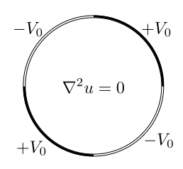
The geometry of the problem is shown below. The capacitor consists of a circular strip of elastic material on which have been patterned four electrodes. Two (the top right and the bottom left) are held at a constant positive voltage; the other are hold at a constant negative voltage. The interior of the capacitor is filled with some dielectric material such as air. The elastic material around the edge has a resistance to both bending and stretching.
Over the course of this sequence of tutorials, we’ll gradually build up our solution. First, we’ll just solve for the electric potential on a fixed shape, and then add in the flexibility later. This practice is recommended when solving new problems with Morpho, so that the program can be robustly tested at each stage.
As a first step, let’s begin by loading an initial mesh for the problem, supplied as “disk.mesh” in the examples folder. Run Morpho and type,
[code gutter=”false” lang=”js”]m=manifoldload("disk.mesh")[/code]
and visualize the mesh by typing,
[code gutter=”false” lang=”js”]show(m)[/code]
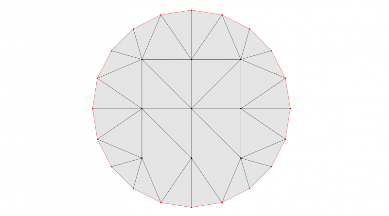
The below mesh will appear in a separate window:
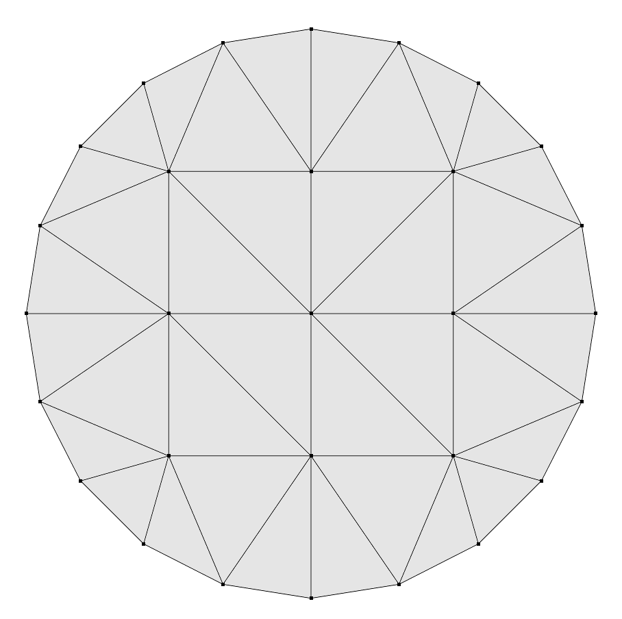
You’ll notice that the mesh is quite coarse in resolution: it has only a few vertices, and the circular boundary appears quite polygonal. During the tutorials, we’ll use Morpho to refine it, adding additional vertices, lines and area elements. This pattern of refinement is very common for solving problems with Morpho.
We will need to refer to specific parts of the mesh during the program such as the overall boundary and the electrodes. To do this, Morpho provides the ability to select subsets of the mesh, and use these selections when doing things like applying energies, etc. Moreover, selections are automatically updated as the mesh is refined. There are several ways to make selections, but one convenient way is to use selectboundary(). Try typing
[code gutter=”false” lang=”js”]boundary=m[1].selectboundary()[/code]
which produces a selection object representing the boundary of the disk. Don’t worry too much about the index m[1] for the moment. As we’ll discuss in later tutorials, it’s necessary here because the selectboundary() selector is actually provided by the underlying manifold object rather than by the body object which provides most functionality that the user typically interacts with.
To check that the selection is referring to the right thing, we can use draw() to visualize the selection:
[code gutter=”false” lang=”js”]show(m.draw(boundary))[/code]
which produces the following:
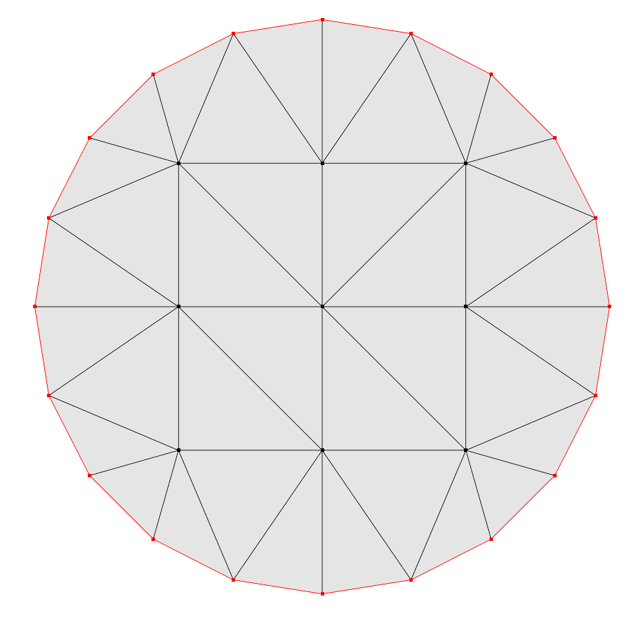
Notice that both the boundary edges and vertices are selected, and highlighted in red. Wherever we need to refer to the boundary later, we can use this selection object that we just created.
To select the electrodes, we can use select() which allows us to filter based on the spatial location of the vertices:
[code gutter=”false” lang=”js”]electrode1=m.select(x^2+y^2>0.99 && ((x>-0.1 && y>-0.05) || (x<0.1 && y<0.05)), coordinates={x,y,z}, grade={0,1});[/code]
There’s quite a lot here, so let’s unpack each of the arguments to select():
The first is a logical comparison that is applied to every element of the mesh. We only want vertices on the boundary, which lies on the line $x^2+y^2=1$. Hence looking for vertices for which $x^2+y^2>0.99$ captures all of the boundary vertices. The other comparisons select out the top right or bottom left respectively. We use cutoff values just below $x=0$ and $y=0$ so that we include vertices right on the boundary in the selection.
The option coordinates={x,y,z} tells morpho that in the first argument, the variables x, y and z refer to the spatial coordinates; we can refer to them by any name we choose.
Finally, grade={0,1} tells morpho to select vertices and line elements. We’ll introduce this nomenclature in a later tutorial, but for now just accept that grade 0 refers to vertices and grade 1 refers to lines.
Exercise 1 Visualize the selection electrode1. Are all the elements you expect included?
Exercise 2 Try changing the parameters of the above call to select(). Can you increase or decrease the number of selected elements? What happens if you change the values in grade? What is selected if you include 2 in the list as well as 0 and 1?
Exercise 3 Can you select the upper and left and bottom right electrodes to make a selection electrode2?
My solution to exercise 3 is below:
[code lang=”js” gutter=”false” collapse=”true” title=”Select electrode2″]
electrode2=m.select(x^2+y^2>0.99 && ((x<0.1 && y>-0.05) || (x>-0.1 && y<0.05)), coordinates={x,y,z}, grade={0,1});
[/code]
In the next tutorial, we’ll define the electric potential, apply energies to the manifold, and perform our first minimization.