Signal Processing in Finance
Signal Processing in Finance
Abstract
With the advent of digital technology and the accompanying gains in processing speed and data storage, techniques in signal processing have become increasingly sought after in the finance industry. These techniques, although traditionally used exclusively in engineering to analyze electrical signals, have proved general enough that their use now transcends engineering and form the basis of any field where time varying signals are subjects of interest. Finance is one such field since financial data is very often compiled with reference to time as the independent variable. More specifically, most forms of time varying financial data may be interpreted as discrete time signals. Not surprisingly, mathematical techniques used in digital signal processing are at present making forays into the finance industry precisely because the problems relating to signals faced by professionals in either field are identical for signals, whether electrical or financial, receive the same treatment in the abstract realm of signal processing.
Introduction
To first understand the relevance of signal processing in finance, it may first be rewarding to explore the concept of a signal itself. A signal is any sequence of numerical data that varies with respect to an underlying independent variable, mostly time. Although the very abstract nature of this definition is exceedingly useful in treating problems from a diverse range of fields, it has historically been applied almost exclusively to problems in electrical engineering. In this field, one encounters a plethora of situations with linear streams of numbers that vary with time. Current and voltage, among others, are obvious examples of this. As an illustration, let us consider the data in Table 1 and its corresponding graph in Figure 1.
Table 1
Table Title. Source: Nepal (2015).
| Time(seconds) | Voltage(Volts) |
|---|---|
| 0 | 10 |
| 1 | 12 |
| 2 | 14 |
| 3 | 8 |
| 4 | 16 |
| 5 | 10 |
| 6 | 12 |
| 7 | 14 |
| 8 | 8 |
| 9 | 16 |
| 10 | 10 |
| 11 | 12 |
| 12 | 14 |
| 13 | 8 |
| 14 | 16 |
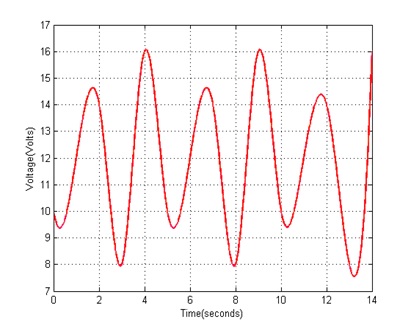
Figure 1
Caption Text. Source: Nepal (2015).
Here, the sequence of numerical data is voltage and it varies with the number of seconds elapsed, i.e. time. Since this data fulfils all the criteria set by the definition above, it is a signal. The table and the graph by themselves provide valuable information about this signal such as its exact value for every second and visualization of its fluctuation. But the diversity and quantity of information directly obtainable from them is fairly limited. This is where signal processing enters the scene to delve into the guts and bowels of a signal to reveal information seldom accessible via a straightforward glance at the data.
While the example of a signal described in Figure 1 is very pertinent to electrical engineering, it may seem out of place in a finance setting. However, all it takes for the preceding example to assume relevance to finance is for one to simply replace the title of the dependent variable from “Voltage” to, for instance, “Daily Earnings” and that of the independent variable to “Day of the Week”. For that matter, the numbers in the table above could be titled in any way possible and yet the mathematical treatment afforded to them would stay identical because the crux of any signal is always in the numbers. This is the central tenet of signal processing in finance because financial data compiled across some duration is hardly distinguishable from voltage or current data seen in an oscilloscope when both are listed on paper. For this reason, the finance industry today stands to benefit profoundly from the fruits of decades of intense research and discoveries in a field only modestly related to it.
Relevance of Signal Processing to Finance
In financial investment strategy, there are two prominent schools of thought: fundamental analysis and technical analysis. The former aims to assess the true value of a business regardless of its transient market value. This approach has limited use for signal processing because it specifically avoids the troves of data such as daily share prices and uses more modest quantities of data for a somewhat subjective assessment. In contrast, at the heart of technical analysis lies the aim of using historical financial data to predict the future market value of a business. This is precisely the type of task for which signal processing is suited because the quantity of historical data is often immense and the sheer objectivity demanded in calculations is scarcely different from that seen in electrical engineering applications.
Signal processing techniques are generally used for technical analysis by major investment banks and especially by hedge funds. The latter, partly because of less government regulation, have very unconventional and secretive investment strategies. Top hedge funds are well known to seek the services of professional engineers and mathematicians to aid them in developing proprietary algorithms that could give them a competitive edge over rivals. This is most often realized by feeding immense quantities of historical share price data to an algorithm that then predicts what direction the prices will move in the near future which can range from seconds to years. Signal processing applied to investments lasting for far shorter durations of literally milliseconds or even micro-seconds is called “High Frequency Trading”. It takes advantage of very momentary random fluctuations in the market to generate reasonable profits on low margins but enormous volumes. Although akin to fortune telling, these strategies are deeply rooted in mathematics and fully rely on electronic equipment to succeed.
Basics of Frequency Domain Analysis, Noise, and Filtering
The Fourier Transform
The mathematical operation known as the “Fourier Transform” occupies an extremely important position in signal processing. The essence of this transform is to take a time varying signal such as described in Figure 1 and deduce any cyclical components present in the signal. For instance, in the signal in Figure 1, it appears that it repeats every 5 seconds because the voltage at t = 0s equals the voltage at t = 5s which in turn equals the voltage at t = 10s. The same may be said for voltages at t = 1s and t = 6s. For a simple signal like this, such periodicity may easily be appreciated from its graph. But for the signal in Figure 2, deduction of periodicity or frequency from the graph alone is difficult.
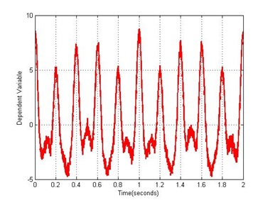
Figure 2
Caption Text. Source: Nepal (2015).
For a signal such as this, there are often multiple frequencies involved and to make matters more intractable, these frequencies may not even be of equal importance. The Fourier Transform tackles this issue by deducing not only what frequencies are present in a signal but also their relative contributions to the signal. This is demonstrated in Figure 3 which shows the Fourier Transform of the signal in Figure 2. From the figure, it is clearly seen that the signal has five distinct frequencies with varying contributions. This ability is crucial in detecting cycles in a signal and once a cycle’s existence has been established, prediction of a future value starts to seem less like fortune telling and much more like objective truth. This concept is absolutely central to technical analysis whose sole purpose rests on analyzing past prices of financial instruments such as stocks to predict their future price.
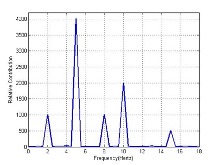
Figure 3
Caption Text. Source: Nepal (2015).
Noise
Another important concept in signal processing is that of noise. An illustration of this can be seen if Figure 2 is compared to Figure 1. The former appears jagged and less smooth than the latter. This is caused by the addition of random numerical values to each data point in Figure 2. Such random values are a natural part of any signal in real life. In electrical engineering, they arise due to slight inconsistencies in the media of transmission (such as air, cables, optical fibers etc.) while in financial data, they are often results of erratic patterns seen in daily trades. Any signal observed in real life can be summarized by the simple equation “observed signal = underlying signal + noise”. The noise component of an observed signal is a signal in its own right but it is intrinsically random and usually rapidly fluctuating, i.e. it has a high frequency. An example of this is illustrated in Figure 4 which contains data for the S&P 500 index for the last 500 trading days (as of February 13, 2015). It may be seen that this signal is relatively noisy because of the frequently occurring steep changes in value and jagged contours. This is a sign of the underlying volatility of the stock market. Such noise is often a hindrance to proper processing of financial data and must be removed. This is usually accomplished with the use of “filters” which are treated next.
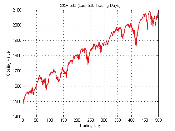
Figure 4
Caption Text. Source: Nepal (2015).
Filtering
It was explained above that the inherent frequencies in a signal may be extracted using the Fourier Transform. This yields valuable information about what stage of the cycle the markets are currently at and approximately how long it will be before they reach the desired stage. A separate procedure effectible with the use of this information is to cancel out certain frequencies while preserving others. This procedure is the essence of filtering and its role in reducing noise from signals is critical. This is made possible by the Fourier Transform because it yields a neat representation of frequencies on the x-axis and their relative strengths on the y-axis. One is then able to retain desirable frequencies and zero out unwanted frequencies before taking the “Inverse Fourier Transform” to return to the time domain signal. In this way, the remaining signal is a “filtered” version of the original signal. Figure 5 demonstrates an example of a “moving average filter”. The x-axis on the plot shown is frequency and the y-axis shows by how much the corresponding frequency is magnified if a signal were to be passed to this filter, i.e. gain. For this filter, the gain is high for lower frequencies but falls off rapidly for higher frequencies.

Figure 5
Caption Text. Source: Nepal (2015).
Filtering is important to signals such as stock market data because of the high volatility of such financial instruments caused by rapid fluctuation in their values. Fortunately, since noise usually fluctuates very rapidly, its frequency is very high. Therefore, when the Fourier Transform of the signal is taken, noise is represented at high frequencies towards the extreme right of the x-axis. A filter can then be applied to reject these high frequencies while preserving the actual signal at low frequencies. This concept is illustrated in Figure 6. The red plot represents the data previously seen in Figure 5 while the blue plot is a filtered version of that data. The filter used here is the “50 Day Moving Average Filter” which is a version of the filter seen in Figure 4. It takes the mean of the closing prices of the S&P 500 of the past 50 days to calculate the value for any given day. This type of filter is known to preserve low frequency signals while getting rid of high frequency signals. While the original signal does display an upward trend, the existence of temporary peaks and deep troughs caused by steep gradients is a major source of distraction to traders. The filtered signal, by contrast, establishes the absoluteness of the upward trend and allows traders to rise above the trivialities of daily market movements in order to appreciate the bigger picture.
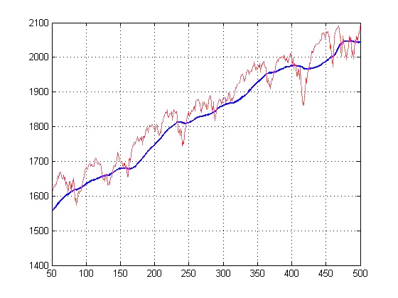
Figure 6
Caption Text. Source: Nepal (2015).
Linear Prediction Filter
A special class of filters used in finance is the linear prediction filter. This filter uses the past values of a signal to predict the next value (Vaidyanathan, 2008). The reason for the effectiveness of linear prediction filters is that signals are rarely completely random and have some degree of consistency of pattern. Linear prediction filters attempt to assess this pattern and yield the most likely future value. When the future value being predicted becomes available, it can be compared against the predicted value and an error estimate may be calculated. The error estimate itself may then be fed back to the filter to improve predictions. This filter is the quintessential tool for a technical analyst trying to conjecture future market swings based on past swings.
An Efficient Algorithm to Compute the Fourier Transform
While the benefits of the Fourier Transform are truly extraordinary, there is the caveat that it is excruciatingly slow to calculate even for a computer. Given that signals in finance (or electrical engineering) can be of truly immense lengths consisting of millions of data points, it is very impractical for today’s computers to compute it. To address this problem, a novel algorithm known as the “Fast Fourier Transform (FFT)” has been discovered. It yields a reasonably workable approximation of a signal’s exact Fourier Transform but takes only a tiny fraction of the time that it takes to compute the Fourier Transform (Briggs et al, 1995). For instance, for a signal with 100 points of data, the FFT is exactly 50 times faster than the conventional method to calculate the Fourier Transform. This comes with the added benefit that the gain in time that the FFT makes possible also increases with the length of the signal. Therefore, for a signal with a million points of data, the FFT is not just 50 but almost 167,000 times faster than the conventional method. The FFT is therefore an indispensable tool in modern signal processing and it has made it possible to use inexpensive electronic devices for rapid calculations.
Devices and Software Used for Financial Signal Processing
Hardware
Personal computers continue to find tremendous use in financial signal processing because of their ubiquity and low costs. Coupled with reasonably fast processing speed and large storage capacity, personal computers are in many ways ideal for signal processing tasks. However, when portability is a factor, specialized digital signal processors (DSP’s) are more useful. This is especially the case for traders who indulge in real time transactions such as on the stock market floor or for professionals who are constantly on the move. DSP’s lack the sheer processing power and storage of personal computers but their electronic structure is so designed as to be dedicated solely to signal processing algorithms.
Software
For signal processing tasks done on personal computers where processing power and storage are rarely of much concern, MatlabTM, produced by Mathworks, is overwhelmingly preferred by professionals not only because of the rapid prototyping of algorithms it allows but also because of software toolboxes that the company has released specifically for signal processing. This means that most of the common algorithms have already been implemented on Matlab and the user’s task is reduced to simply knowing what algorithm to use in what situation. However, since Matlab is a high level language in that it does not allow direct control of the hardware it is implemented on, it is difficult to optimize its performance specific to portable DSP’s. For this reason, when signal processing has to be implemented remotely, as is the case for traders on the floor, algorithms are usually designed to optimize the available hardware using a low level language such as C which confers far more influence over hardware to the programmer.
Regardless of the selection of software applications used to implement the algorithms, the algorithms themselves are drawn directly from mathematics. Numerous mathematicians since Joseph Fourier’s breakthrough in Fourier series in 1807 have directly contributed to signal processing in the last 200 years. The follow up on Fourier series by Dirichlet, the work on information theory by Shannon, and the discovery of the FFT algorithm by Cooley and Tookey all rank as major developments in signal processing. Even before Fourier himself, the likes of Lagrange and Gauss had inadvertently made mathematical contributions that would lead to the modern concept of signal processing (Heideman et al, 1984). Other areas of mathematics such as linear algebra contain valuable tools for signal processing because of the generality of their applications. Also important are topics from probability and statistics because the inherently noisy nature of real life signals requires probabilistic models and statistical measures. At the forefront lie topics such as neural networks which, instead of using deterministic algorithms, try to mimic biological systems of neurons to learn and modify algorithms without human interference (Kahn et al, 1995). Although long limited on paper for lack of sufficient digital technology, these theoretical breakthroughs became practical with the advent of computers in the latter half of the 20th century thanks to Moore’s Law and the change has especially accelerated since the 1990s.
Bibliography
- Briggs, W. L., & Henson, V. E. (1995). The DFT: An owner’s manual for the discrete Fourier transform. Philadelphia: Society for Industrial and Applied Mathematics. OCLC WorldCat Permalink: http://www.worldcat.org/oclc/31938467
- Heideman, M., Johnson, D. H., & Burrus, C. S. (1984). Gauss and the history of the fast fourier transform. IEEE ASSP Magazine, 1(4), 14–21. DOI: 10.1109/MASSP.1984.1162257
- Kahn, R. N., & Basu, A. K. (1995). Neural networks in finance: an information analysis. In Computational Intelligence for Financial Engineering, 1995., Proceedings of the IEEE/IAFE 1995 (pp. 183–191). DOI: 10.1109/CIFER.1995.4952
- Vaidyanathan, P. P. The Theory of Linear Prediction. San Rafael, Calif.: Morgan & Claypool, 2008. OCLC WorldCat Permalink: http://www.worldcat.org/oclc/840401216
All data and figures used were produced by Nepal (2015) with Microsoft-Excel 2013 and Matlab 2010.
Suggested Reading
- “The Origins of the Sampling Theorem” Luke, H.D., 1999
- “Sampling, data, and the Nyquist Rate” Landau, 1967