Sometimes My Head Hurts: Internal Consistency and Statistical Power

Sometimes My Head Hurts

Co-authors and I received a desk reject of a manuscript earlier this week, but that’s not why my head hurts. My head hurts because I’ve been trying to wrap it around the concept of reliability, specifically internal consistency reliability. Why? Because one of the reasons for the desk reject was a question about the reliability of our measures in the study. Allow me to explain.

The Study

The amazing Sarah Cavanagh came up with a great idea for a study, together with Jim Lang, Jeff Birk, and Carl Fulwiler. Specifically, we sought to determine whether training college students some skills related to mindfulness and emotion regulation in the classroom – and I mean literally in the classroom – would improve their learning. Long story short, we did this [^1] by delivering two interventions and an instructional control condition using a slew of iPads over the course of two semesters in three different classes. You can find a description in our preregistration. For the moment, the key point is that each student received all three interventions on different class days and they took a quiz each time about the day’s lesson.

Our hypothesis was that the interventions would each lead to better learning than the instructional control condition. This meant testing whether quiz scores in each intervention condition were higher than quiz scores in the control condition. Because every student completed both conditions, this is a within-subjects comparison that can be examined using a paired t-test. [^2]

Measurement reliability is a key to the statistical power of this (and any) test. Statistical power is the probability of detecting a true effect. If there is a true effect to detect, then we definitely want to detect it so how can we assess the reliability of our quiz scores?

Internal Consistency Reliability

When one has a set of items all purporting to assess the same construct (like a quiz purporting to assess learning), internal consistency reliability is sensible to assess. When internal consistency reliability is calculated for a set of items (columns) in a sample of people (rows), it basically tells us to what extent people who score higher (or lower) on one item also score higher (or lower) on other items. It’s an indicator of how good we are at distinguishing the scores of individual participants. If we can’t distinguish the scores of different individuals, then we can’t know for sure that something we have done to those individuals (like delivering an iPad intervention in the classroom) has had an impact.

Ultimately, of course, we care about individuating students based on overall scores across items. Assessments of internal consistency reliability of the items that go into the overall score tell us how good a job we’re doing at that. In the ideal scenario, the rank order of scores for different participants would be the same each time, regardless of which intervention condition they’re experiencing (i.e., Student A scores higher than Student B who scores higher than Student C on every quiz). The less reliable that ranking, the harder it is to detect a difference between the conditions (i.e., we have less statistical power to detect true effects).

This bring us back to my head hurting. It’s not hurting because we need to assess reliability. It’s hurting because R.

Wherefore R(t) Thou

I got curious about how, exactly, internal consistency reliability affects statistical power for a paired t-test. I wanted to see with my own two eyes the answer to this question: How does statistical power – measured as the proportion of times p < .05 out of 1,000 repetitions – scale with internal consistency reliability? Specifically, I wanted to know how different levels of internal consistency impact statistical power to detect a within-subjects difference of 5% (half a letter grade) between two quiz scores (75% in one condition and 70% in the other). To answer this question, I spent some time [^3] working on simulations in R. I set it up to repeat the following steps 1,000 times:

Generate two sets of 5 dichotomous items – 1 for correct, 0 for incorrect – for each of 140 participants with different levels of internal consistency from low (0.00) to high (1.00),
Compute the mean for each quiz, and then
Run a paired t-test to see if the difference is statistically significant at p < .05.

Here’s the code: (Updated some error corrections and improvements on 2018 July 9)

# Impact of internal consistency reliability of a set of items
# on power to detect significant mean differences in a t-test 
# comparing two conditions, C1 and C2, on a mean across items.

############################################################
#user needs to specify the following:

# set desired correlation(s) between simulated items
# can be a range of values; the script will loop as 
# many times as there are entries
itemcor <- seq(0, 1, .05) # this sets sequence from 0 to 1 by increments of .05

# set desired number of participants
np <- 140 

# set desired total number of items *across two conditions* (5 items each = 10)
# code will loop through more than once if more than one ni value is entered here
ni <- c(6,10)

# set number of simulations
numrep <- 1000

# set desired mean proportion correct in C1 and C2 conditions
C1 <- .75
C2 <- .70
SD <- .25 #assuming the standard deviation is the same in both conditions

# set whether this a paired t-test (options: TRUE, FALSE)
paired <- TRUE

# do you want dichotomous items? (1=yes, 0=no)
# code will loop through more than once if more than one dichot value is entered here
dichot <- c(0,1)


# set working directory
#setwd("U:/07_blog_emotiononthebrain/Internal Consistency")


############################################################

# call libraries
library(multilevel)
library(tidyr)
library(MBESS)
library(psych)
library(ggplot2)
library(effsize)
library(viridis)
library(animation) # must install ImageMagick outside of R first
library(magick)
library(gridExtra)


for(d in 1:length(dichot)){ # type of items loop

  for(n in 1:length(ni)){  #number of items loop

    # initialize indexes
    index <- 0
    col1 <- 2
    col2 <- ni[n]/2 + 1
    col3 <- 2 + (ni[n]/2)
    col4 <- ni[n] + 1

    # determine plot number
    plotnum <- paste("powercurve_d",d,"n",n,sep="")

    # initialize reliability output file
    reliability <- data.frame()

    for(i in 1:length(itemcor)){

      for(j in 1:numrep){

      # simulate specified # of items that are correlated by amount noted above
      data <- sim.icc(gsize=np,ngrp=1,nitems=ni[n],item.cor=itemcor[i],icc1=0)

      # rescale to desired mean and SD
      data1 <- rescale(data[col1:col2], mean=C1, sd=SD)
      data2 <- rescale(data[col3:col4], mean=C2, sd=SD)
      subject <- data.frame(row.names(data1))
      data <- cbind(subject,data1,data2)
      names(data)[1] <- "subject"

      # restructure the file to be long
      data_long <- gather(data, key = "trial", value = "correct", col1:col4)

      data_long1 <- data_long[1:(nrow(data_long)/2), ]
      data_long2 <- data_long[((nrow(data_long)/2)+1):nrow(data_long), ]

      if (dichot[d] == 1){
        # convert col1 to col2 vars to values of 0 and 1 (C1)
        data_long1$correct[ data_long1$correct > quantile(data_long1$correct,probs=1-C1)[[1]] ] <- 1
        data_long1$correct[ data_long1$correct <= quantile(data_long1$correct,probs=1-C1)[[1]] ] <- 0

        # convert col3 to col4 vars to values of 0 and 1 (C2)
        data_long2$correct[ data_long2$correct > quantile(data_long2$correct,probs=1-C2)[[1]] ] <- 1
        data_long2$correct[ data_long2$correct <= quantile(data_long2$correct,probs=1-C2)[[1]] ] <- 0
      }

      # set condition variables
      data_long1$GRP <- .5
      data_long2$GRP <- -.5

      # concatenate the two files vertically
      data_long <- rbind(data_long1,data_long2)

      if (dichot[d] == 0){
        # set max correct to 1 and min correct to 0
        data_long$correct[ data_long$correct > 1 ] <- 1
        data_long$correct[ data_long$correct <= 0 ] <- 0
      }

      # create wide file for paired t-test
      data_agg <- aggregate(x = data_long$correct, by = list(data_long$subject,data_long$GRP), FUN = mean)
      names(data_agg)[1] <- "subject"
      names(data_agg)[2] <- "GRP"
      names(data_agg)[3] <- "Mscore"
      data_agg_spread <- spread(data_agg,key="GRP",value="Mscore")
      data_agg_spread$"C1-C2" <- data_agg_spread$"0.5"-data_agg_spread$"-0.5"

      # report descriptives for each condition
      reliability[j+index,"M C1"] <- mean(data_agg_spread$"0.5")
      reliability[j+index,"SD C1"] <- sd(data_agg_spread$"0.5")
      reliability[j+index,"M C2"] <- mean(data_agg_spread$"-0.5")
      reliability[j+index,"SD C2"] <- sd(data_agg_spread$"-0.5")
      reliability[j+index,"C1-C2"] <- mean(data_agg_spread$"C1-C2")
      reliability[j+index,"SD C1-C2"] <- sd(data_agg_spread$"C1-C2")
      reliability[j+index,"d"] <- cohen.d(data_agg_spread$"0.5",data_agg_spread$"-0.5",paired=paired)$estimate

        # calculate Cronbach's alpha
      alpha.data_C1 <- ci.reliability(data=data[ ,col1:col2], 
                                      type="alpha", 
                                      interval.type="none")$est 

      alpha.data_C2 <- ci.reliability(data=data[ ,col3:col4],  
                                      type="alpha", 
                                      interval.type="none")$est 
      reliability[j+index,"Cronbach's alpha C1"] <- alpha.data_C1
      reliability[j+index,"Cronbach's alpha C2"] <- alpha.data_C2

      reliability[j+index,"itemcor"] <- itemcor[i]

        # calculate correlation between overall scores in the two conditions
      reliability[j+index,"r"] <- cor(data_agg_spread[2],data_agg_spread[3])[[1]]

      # compute paired t-test and extract values of interest
      reliability[j+index,"t"] <- t.test(data_agg_spread$"0.5", data_agg_spread$"-0.5", data=data_agg_spread, paired=paired)$statistic[[1]]
      reliability[j+index,"p"] <- t.test(data_agg_spread$"0.5", data_agg_spread$"-0.5", data=data_agg_spread, paired=paired)$p.value

      # print info about which loop we're in to facilitate monitoring progress
      print(paste0("dichot: ", dichot[d],",  items: ", ni[n]/2,", itemcor: ", itemcor[i],", rep: ", j))

      } #end j loop

      # update index so that values in next loop are recorded in the correct row
      index <- index+numrep
    } # end i loop

    # figure out how many p values are below .05
    reliability$sig[ reliability$p < .05] <- 1

    # summarize proportion of significant mean diffs
    result <- data.frame(table(reliability$itemcor, reliability$sig))
    result$sigprop <- result$Freq/numrep
    names(result)[1] <- "itemcor"

    # summarize median descriptives and Cronbach's alpha for each itemcor
    result2 <- aggregate(x = reliability[1:13], 
                         by = list(reliability$itemcor), 
                         FUN = median)
    if(nrow(result)==0){result[1:nrow(result2),"sigprop"] <- NA} # handles empty result data frame
    result2 <- cbind(result2, result$sigprop)
    names(result2)[15] <- "sigprop"


    #graph power curve
    alpha <- data.frame(result2
Sometimes My Head Hurts


Co-authors and I received a desk reject of a manuscript earlier this week, but that's not why my head hurts. My head hurts because I've been trying to wrap it around the concept of reliability, specifically internal consistency reliability. Why? Because one of the reasons for the desk reject was a question about the reliability of our measures in the study. Allow me to explain.

The Study


The amazing Sarah Cavanagh came up with a great idea for a study, together with Jim Lang, Jeff Birk, and Carl Fulwiler. Specifically, we sought to determine whether training college students some skills related to mindfulness and emotion regulation in the classroom - and I mean literally in the classroom - would improve their learning. Long story short, we did this [^1] by delivering two interventions and an instructional control condition using a slew of iPads over the course of two semesters in three different classes. You can find a description in our preregistration. For the moment, the key point is that each student received all three interventions on different class days and they took a quiz each time about the day's lesson.

Our hypothesis was that the interventions would each lead to better learning than the instructional control condition. This meant testing whether quiz scores in each intervention condition were higher than quiz scores in the control condition. Because every student completed both conditions, this is a within-subjects comparison that can be examined using a paired t-test. [^2]

Measurement reliability is a key to the statistical power of this (and any) test. Statistical power is the probability of detecting a true effect. If there is a true effect to detect, then we definitely want to detect it so how can we assess the reliability of our quiz scores?

Internal Consistency Reliability


When one has a set of items all purporting to assess the same construct (like a quiz purporting to assess learning), internal consistency reliability is sensible to assess. When internal consistency reliability is calculated for a set of items (columns) in a sample of people (rows), it basically tells us to what extent people who score higher (or lower) on one item also score higher (or lower) on other items. It's an indicator of how good we are at distinguishing the scores of individual participants. If we can't distinguish the scores of different individuals, then we can't know for sure that something we have done to those individuals (like delivering an iPad intervention in the classroom) has had an impact.

Ultimately, of course, we care about individuating students based on overall scores across items. Assessments of internal consistency reliability of the items that go into the overall score tell us how good a job we're doing at that. In the ideal scenario, the rank order of scores for different participants would be the same each time, regardless of which intervention condition they're experiencing (i.e., Student A scores higher than Student B who scores higher than Student C on every quiz). The less reliable that ranking, the harder it is to detect a difference between the conditions (i.e., we have less statistical power to detect true effects).

This bring us back to my head hurting. It's not hurting because we need to assess reliability. It's hurting because R.

Wherefore R(t) Thou


I got curious about how, exactly, internal consistency reliability affects statistical power for a paired t-test. I wanted to see with my own two eyes the answer to this question: How does statistical power - measured as the proportion of times p < .05 out of 1,000 repetitions - scale with internal consistency reliability? Specifically, I wanted to know how different levels of internal consistency impact statistical power to detect a within-subjects difference of 5% (half a letter grade) between two quiz scores (75% in one condition and 70% in the other). To answer this question, I spent some time [^3] working on simulations in R. I set it up to repeat the following steps 1,000 times:



 	Generate two sets of 5 dichotomous items - 1 for correct, 0 for incorrect - for each of 140 participants with different levels of internal consistency from low (0.00) to high (1.00),


 	Compute the mean for each quiz, and then


 	Run a paired t-test to see if the difference is statistically significant at p < .05.




Here's the code: (Updated some error corrections and improvements on 2018 July 9)
Cronbach's alpha C1`,result2

Sometimes My Head Hurts


Co-authors and I received a desk reject of a manuscript earlier this week, but that's not why my head hurts. My head hurts because I've been trying to wrap it around the concept of reliability, specifically internal consistency reliability. Why? Because one of the reasons for the desk reject was a question about the reliability of our measures in the study. Allow me to explain.

The Study


The amazing Sarah Cavanagh came up with a great idea for a study, together with Jim Lang, Jeff Birk, and Carl Fulwiler. Specifically, we sought to determine whether training college students some skills related to mindfulness and emotion regulation in the classroom - and I mean literally in the classroom - would improve their learning. Long story short, we did this [^1] by delivering two interventions and an instructional control condition using a slew of iPads over the course of two semesters in three different classes. You can find a description in our preregistration. For the moment, the key point is that each student received all three interventions on different class days and they took a quiz each time about the day's lesson.

Our hypothesis was that the interventions would each lead to better learning than the instructional control condition. This meant testing whether quiz scores in each intervention condition were higher than quiz scores in the control condition. Because every student completed both conditions, this is a within-subjects comparison that can be examined using a paired t-test. [^2]

Measurement reliability is a key to the statistical power of this (and any) test. Statistical power is the probability of detecting a true effect. If there is a true effect to detect, then we definitely want to detect it so how can we assess the reliability of our quiz scores?

Internal Consistency Reliability


When one has a set of items all purporting to assess the same construct (like a quiz purporting to assess learning), internal consistency reliability is sensible to assess. When internal consistency reliability is calculated for a set of items (columns) in a sample of people (rows), it basically tells us to what extent people who score higher (or lower) on one item also score higher (or lower) on other items. It's an indicator of how good we are at distinguishing the scores of individual participants. If we can't distinguish the scores of different individuals, then we can't know for sure that something we have done to those individuals (like delivering an iPad intervention in the classroom) has had an impact.

Ultimately, of course, we care about individuating students based on overall scores across items. Assessments of internal consistency reliability of the items that go into the overall score tell us how good a job we're doing at that. In the ideal scenario, the rank order of scores for different participants would be the same each time, regardless of which intervention condition they're experiencing (i.e., Student A scores higher than Student B who scores higher than Student C on every quiz). The less reliable that ranking, the harder it is to detect a difference between the conditions (i.e., we have less statistical power to detect true effects).

This bring us back to my head hurting. It's not hurting because we need to assess reliability. It's hurting because R.

Wherefore R(t) Thou


I got curious about how, exactly, internal consistency reliability affects statistical power for a paired t-test. I wanted to see with my own two eyes the answer to this question: How does statistical power - measured as the proportion of times p < .05 out of 1,000 repetitions - scale with internal consistency reliability? Specifically, I wanted to know how different levels of internal consistency impact statistical power to detect a within-subjects difference of 5% (half a letter grade) between two quiz scores (75% in one condition and 70% in the other). To answer this question, I spent some time [^3] working on simulations in R. I set it up to repeat the following steps 1,000 times:



 	Generate two sets of 5 dichotomous items - 1 for correct, 0 for incorrect - for each of 140 participants with different levels of internal consistency from low (0.00) to high (1.00),


 	Compute the mean for each quiz, and then


 	Run a paired t-test to see if the difference is statistically significant at p < .05.




Here's the code: (Updated some error corrections and improvements on 2018 July 9)
Cronbach's alpha C2`)
    x <- rowMeans(alpha)
    y <- result2$sigprop
    graphpc <- data.frame(x,y)

    p <- ggplot(graphpc, aes(x, y)) + geom_point() + theme_classic() +
      scale_x_continuous(limits=c(-.05,1),breaks = seq(0, 1, .1)) +
      scale_y_continuous(limits=c(0,1),breaks = seq(0, 1, .2)) +
      geom_smooth(method = "gam", formula = y ~ poly(x, 2), se = FALSE) +
      geom_hline(yintercept = .80, linetype="dotted") +
      {if(paired)annotate("text", x = .5, y = .78, label = "paired t-test" )} + 
      {if(!paired)annotate("text", x = .5, y = .78, label = "independent t-test" )} + 
      annotate("text", x = .2, y = .10, label = paste("median M diff =", sprintf("%0.2f", round(median(result2$"C1-C2"),digits=2))) ) +
      annotate("text", x = .2, y = .05, label = paste("SD M diff =", sprintf("%0.3f", round(max(result2$"SD C1-C2"),digits=3)),"to", sprintf("%0.3f", round(min(result2$"SD C1-C2"),digits=3)),"(left to right)") ) +
      annotate("text", x = .2, y = .0, label = paste("N =", np) ) +
      ylab(paste("power based on",numrep," simulations")) +
      {if(dichot[d]==0)xlab(paste("Cronbach's alpha based on",ni[n]/2,"continuous items per condition"))} + 
      {if(dichot[d]==1)xlab(paste("Cronbach's alpha based on",ni[n]/2,"dichotomous items per condition"))} + 
      NULL

    # rename plot p to according to string variable, plotnum
    assign(plotnum, p)

    # save the plot to disk with name specific to user input
    if(dichot[d]==1){
      ggsave(paste("powercurve_","Np",np,"_Ni",ni[n]/2,"_dichotomous_C1M",C1,"_C2M",C2,"_SD",SD,"_paired",paired,".png",sep=""),device="png")
    }

    if(dichot[d]==0){
      ggsave(paste("powercurve_","Np",np,"_Ni",ni[n]/2,"_continuous_C1M",C1,"_C2M",C2,"_SD",SD,"_paired",paired,".png",sep=""),device="png")
    }

    #print(eval(as.name(plotnum)))

  } # end n loop
} # end d loop

Yeesh. But it works.

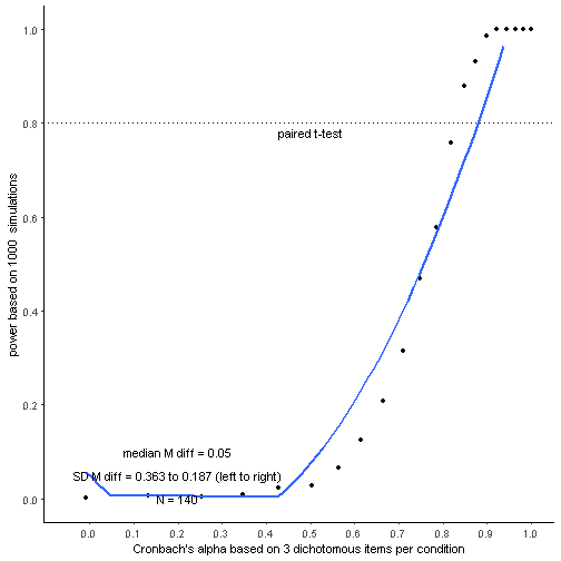
You can see the power curve in the figure below. This power curve is specific to the number of quiz items, the size of the difference between conditions, and the number of participants. But it illustrates the point nicely: As internal consistency reliability increases, so does statistical power. Shazam.

As shown above, with five dichotomous items, we’d achieve at least 80% power to detect predicted differences at all levels of internal consistency reliability, assessed using Cronbach’s alpha (technically, the x axis shows median Cronbach’s alpha averaged across conditions and across all 1,000 simulations). You can also see that the higher the Cronbach’s alpha, the more power you get up to about Cronbach’s alpha = .70, at which point power asymptotes at 1.

However, below you can see what happens when all settings are the same but we have only three instead of five dichotomous items. In this case, we’d need Cronbach’s alpha in the .80 range in order to achieve at least 80% power. And power doesn’t asymptote at 1 until you get up to about Cronbach’s alpha = .90.

What if the items are continuous rather than dichotomous?

I’m glad you asked. Whether you have three or five of them, continuous items afford bunches more statistical power at all levels of internal consistency reliability tested, as you can see below, respectively.

What do the data actually look like at different levels of reliability?

Check out this animated gif, which I have to say I’m damn proud of having made. It displays results for a series of single simulated studies, each with the specs noted above: two paired conditions separated by a mean difference of 5%, steadily increasing reliability, and 5 items. But I’m displaying 30 participants and using continuous items to make the point visually clearer. Here’s what we get (you might have to click it to animate):

What you see are lines connecting the mean scores in each of the two conditions for all individual participants, who are depicted in different colors. As the correlation between the mean score for C1 and the mean score for C2 increases – a byproduct of increasing internal consistency – two things happen: 1) the standard deviation between individuals increases but 2) the standard deviation of the difference between individuals decreases. And as the standard deviation of the difference between conditions decreases, the t value goes up, even with no change in the mean difference between conditions. That’s because the standard deviation of the difference contributes to the denominator used to calculate t, which is what gives the test greater power: The higher t value, the more surprising it would be if the null hypothesis of no difference were true, which is captured in a lower p value.

Of course, the reality is that we wouldn’t expect students to stay in their rank order from quiz to quiz; as Sarah noted in an email exchange, “some topics are learned better or worse by some students, and… students move around quite a lot in their exam scores over a semester – e.g., students in intro who crash and burn during research methods but shine on the biological section, or vice-versa, for instance.” Totally true. And to the extent that this is the case, it will be harder to detect a significant difference between performance on the quiz covering research methods versus performance on the quiz covering the biological material. That’s because the standard deviation of the mean difference will be higher.

Conclusion

If you want to maximize your ability to detect an experimental effect, get you some reliability! As shown in this post, increasing the number of items on your dependent variable is one sure way to do so. Another ways is to use continuous rather than dichotomous items when possible. I only documented a limited range of factors of interest here. For example, the power curves always included 140 participants, and assumed that the reader is interested in a mean difference of only 5% between quizzes comprised of three or five items for a within-subjects comparison. That’s because these are the relevant factors for our intervention study examining mindfulness and emotion regulation in the classroom. Feel free to adapt the R code, which is available here, to your particular context.

If you have any pointers to other resources for documenting associations between reliability and power, feel free to share them in the comments below or hit me up on Twitter @HeatherUrry.

[^1]: When I say “we did this”, what I really mean is that Sarah did this along with Jim and some awesome grad fellows at Assumption College. I understand it was exhausting.
[^2]: I’m simplifying things for expository purposes here; there’s more going on with the design of this study than is relevant to the point I want to make in this post.
[^3]: OK, a lot of time.

Studying the brain and body correlates of emotion, from reaction to regulation

Studying the brain and body correlates of emotion, from reaction to regulation

Sometimes My Head Hurts: Internal Consistency and Statistical Power